Unpacking K-P Flow:
The Geometry of GD Learning in General Recurrent Models
| Relevant Links | |
| Arxiv Pre-Print | Pip Pytorch Package |
TLDR
Q: Can we track the evolution of a dynamical system trained by Gradient Descent (GD)?
A: Yes, but the NTK involves tensor calculus. We need new geometric intuition and dynamical tools.
Synopsis
This blog post provides a more intuitive exploration of some parts of our main paper, linked above, which broadly explores the gradient flow of general recurrent models.
An efficient and in-development package with examples is linked above. See accompanying blog posts on my main page exploring specific aspects of the code.

Fig 1 Poster overview.
Broader Motivation and Prior Work
Recurrent Models in Neuroscience and ML Recurrent models in machine learning are a powerful tool that can mimic sequential behavior when fit to data. Practically, this can be used to solve a variety of tasks in deep learning and control. Furthermore, such models can be used as a proxy for understanding how circuity in the brain forms so-called neural manifolds, consisting of low-dimensional dynamical motifs such as fixed points and attractors. In multi-task learning contexts, recurrent models give insights solving complex continual learning or compositional problems.
Many, Many Recurrent Architectures Classically, in control, the most common recurrent model is the Linear Time Invariant (LTI) controller, which is a linear dynamical system that can be trained on a variety of problems and is well analyzed theoretically. In deep learning, the most classical model is the Recurrent Neural Network (RNN), with non-linear time-stepping dynamics. Building on this model are GRUs and LSTMs, which train better, avoiding pitfalls of vanishing and exploding gradients. More recently, there are many diverse recurrent architectures in deep learning, including those with dynamical synapses (MPNs) or State-Space Models (SSMs). Outside of these contexts, we can look to physics and neuroscience to see a very wide range of complex network-based recurrent dynamical systems, such as spin-glasses, Hodgkin-Huxley biophysical neural networks, Hopfield neural networks, energy-based models, and many, many more.
Training Recurrent Models In control and deep learning, the primary means of "training" such recurrent models is dynamically adapting their parameters (typically weights of the recurrent or output connections) with (potentially stochastic or accelerated) Gradient Descent (GD). More specifically, on discrete models like RNNs or GRUs, we use Backpropagation Through Time (BPTT) to efficiently compute gradients, which are then used to incrementally adjust the parameters. In optimal control or continuous Neural ODEs, this may be instead be labeled as the adjoint method, but it was proven long ago that BPTT and the adjoint method are exactly the same thing.
Tracking Trained Dynamics In this study, we investigated how the dynamics of a recurrent model trained with GD evolve. More specifically, we define operators that, when composed together, define the hidden-state gradient flow of the a general parameterized recurrent dynamical system.
Introduction
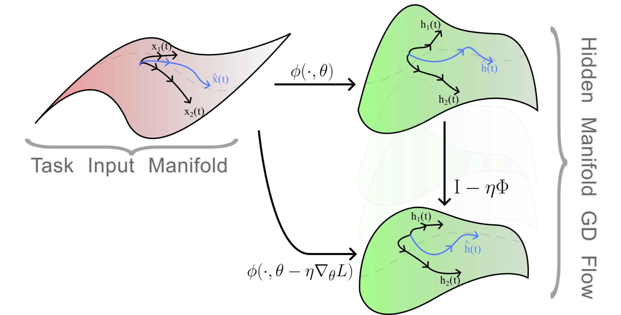
Fig 2 Schematic of network model \(\phi(x, \theta)\), which produces a hidden state over time given input \(x\) and parameters \(\theta\). The hidden state gradient flow (right) describes how the trajectories \(h_j(t)\) evolve. Here, \(\hat x(t)\) is an unseen input during training, and \(\hat h(t)\) is the corresponding hidden state.
Gradient Descent (GD) Setup
A General Recurrent Model As described, we consider a recurrent dynamical system, trained with GD to approximately mirror target trajectories given a variety of time-varying inputs. We let \(h(t)\) denote the model's hidden state, and \(x(t)\) denote a sample task input. The variable \(t\) denotes the forward pass time and exists in a given time range \([0, t_{end}]\). During the forward-pass inference, an individual task input is chosen, \(x(t)\), from a given distribution of all task inputs; then, the model state \(h(t)\) is simulated from an initial state \(h_0\) to time \(t_{end}\), driven by the input \(x(t)\). The dynamics can be continuously specified or discretely with little change in the mathematics below, so we use assume time is continuous. In this case, the model dynamics take the form: $$\frac{d}{dt} h(t) = f(h(t), x(t), \theta), \text{ for } t \in (0, t_{end}]; \text { with } h(0) = h_0.$$ Here, \(\theta\) denote the model parameters (e.g., weights and biases) and \(f\) models the tangential dynamics of the hidden state.
Defining the Task For each input \(x(t)\) we associate and desired output target \(y^*(t)\). Furthermore, we define an output function of the hidden state, e.g., the simple affine map: $$y(t) = W_{out} h(t) + b_{out}.$$ Then, the goal is to minimize a loss function \(\ell(y(t), y^*(t))\) on all possible inputs and at all times. In particular, we define the loss as an average (denoted by \(\langle \cdot \rangle_{x,t}\)): $$L := \langle \ell(y(t), y^*(t)) \rangle_{x,t}.$$
Training the Model with GD The goal is to minimize the loss \(L\) by tuning the parameters of the model, \(\theta\). To do so, we want to find the best parameters: $$\theta^* := \arg \min_\theta L.$$ This is typically done by GD, where the parameters are iteratively updated by travelling down the steepest direction in Euclidean parameter space. Specifically, letting \(\delta \theta\) be the perturbation to the parameters at a particular instant in GD, it is given by: $$\delta \theta := -\eta \nabla_\theta L.$$ Here, \(\eta\) is a learning rate, which I'll just assume is \(1\) throughout the rest of this blog for simplicity.
The Hidden State GD Flow
Tracking the GD Flow We would like to track certain quantities as they evolve under GD. The simplest quantity to track are the parameters, defining the so-called parameter GD flow. However, this quantity is ultimately a proxy for the actual dynamics of the hidden state, which also evolves as GD trains the model. We would like to track how this quantity itself evolves in a meaningful way. The hidden state dynamics can be envisioned as a large vector field, conditioned on the particular input you give the model.
Now, before getting into the details of the objects involved, the general idea (which turns out to work correctly) is simply as follows. Firstly, define the Instantenous Error Signal, Err, by $$\text{Err} := \nabla_{h} \ell(y, y^*).$$ For example, when we use a squared error loss, \(\ell(y, y^*) := \| y - y^*\|\), the error signal is \(\text{Err} = W_{out}^T (y - y^*)\), a simple residual projected onto the row space of \(W_{out}\). Then, by the chain rule, $$\nabla_\theta L = (\frac{d h}{d \theta})^T \text{Err}.$$ Given this small parameter change, the hidden state itself will approximately change linearly by $$\delta h = -\frac{d h}{d \theta} \cdot \nabla_\theta L = -\frac{d h}{d \theta} \cdot \frac{d h}{d \theta}^T \text{Err}.$$ In this blog, I will refer to the Jacobian outer product \(\Phi := \frac{d h}{d \theta} \cdot \frac{d h}{d \theta}^T\) as the Neural Tangent Operator (NTO).
The Neural Tangent Operator
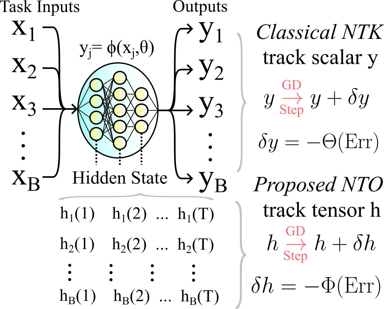
Fig 3 The NTO and NTK for a scalar-output multi-layer-perceptron neural network. The classical NTK \(\Theta\) is a matrix quantifying how GD changes align over batch inputs. By contrast, the NTO \(\Phi\) measures how the activations at every layer change.
I use the non-standard term "neural tangent operator" (NTO) to distinguish this from the classical Neural Tangent Kernel (NTK). The classical NTK is a matrix tracking how the output of a scalar-output multi-layer-perceptron neural network evolves as we train the weights and biases. This NTK is a matrix of shape [B, B], where B is the number of batch inputs on which we evaluate the model and adjust it. In contrast, the NTO for this model would track how all hidden activations, \(h(t)\) for each layer \(t\), evolve over gradient descent. It would be a tensor of shape [T, B, B, T], or, if we vectorize, a matrix of shape [B*T, B*T], so it is much larger. We could also refer to the NTO as the "full NTK," "extended NTK," or "hidden state NTK" I just chose Neural Tangent Operator to make it clear that it is much larger and typically operates on multi-dimensional things, not just vectors. Below I detail this more.
The Classical NTK In the classical NTK literature, the model considered is a multi-layer perceptron neural network with scalar output, so there is no notion of time, \(t\), and no spatial (hidden unit) dimension. Hence, the NTK is just a B by B matrix over all batch input trials. The NTK entries pinpoint how much a GD corrections correlate over batch trials: do corrections to the parameters proposed by two distinct task inputs agree, not overlap at all, or disagree, leading to loss when we do the actual parameter update. I will use the notation \(\Theta\) to denote the NTK. Concretely, if \(y = w^T h\) where \(w\) is a vector, then we can relate the NTO, \(\Phi\), and NTK, \(\Theta\): $$\Theta = w^T \Phi w,$$ i.e. the NTO is the actually complicated part of the whole operator.
The NTO is a tensor operator In our case, however, the NTO is actually a tensor operator. In a Pytorch implementation, for example, the hidden state will have the form [B, T, H] over batch inputs, \(x\), times, \(t\), and hidden units. The quantity \(\frac{d h}{d \theta}\) thus has the form [B, T, H, M], where \(M\) is the size of the flattened model parameters. Finally, \(\Theta\) is an linear operator on the space of tensors of the form [B, T, H]. If we discretize it, it will be a massive matrix of shape B*T*H by B*T*H. If indexed in Pytorch, the of \(\Phi\) are given by $$\Phi: \mathbb{R}^{B\times T \times H} \rightarrow \mathbb{R}^{B \times T \times H}$$ $$\Phi[b, t, h, b_0, t_0, h_0] = \sum_{m=1}^M \frac{d h}{d \theta}[b, t, h, m] \frac{d h}{d \theta}[b_0, t_0, h_0, m].$$ Formally, this is a tensor product on \(\frac{d h}{d \theta}\) where the parameter dimension is contracted (see my blog post going into more depth on tensor calculus). The fact that the NTO is a tensor operator for such general recurrent models has pros and cons. Pros include that it encapsulates a massive amount of information, including insights into GD learning at very granular levels given by eigenfunctions. Indeed, in the next section I'll discuss some of the ways we can reduce the operator to generate different perspectives on the GD learning. However, this is also a since it makes the whole object harder to understand, requiring some tensor math. Another major con is the massive size of this object. Even for very small problems it can be huge (e.g. 100 neurons, batch size 100 and 100 forward-pass times results in \(\Phi\) being 1m by 1m when discretized). Thus, advanced matrix-free methods that do not actually compute the full discretized operator are needed to work with \(\Phi\) (see my blog using trace estimation for the NTO, for example).
Optional: Working with Tensor Operators
The following sections describes how to work with these tensor operators, providing some intuition and a heirarchy of reduced operators. However, it's not entirely necessary for understanding the methods and I may flesh it out in its own post in the future, feel free to skip!
As mentioned in the prior section, the full empirical NTO for recurrent models is a linear operator on a space of 3-tensors (discretely of shape [B, T, H]). In this section, I'll discuss building some more intuition and practical tools for working with such operators. Indeed, it may be tempting to think that working with such a massive, complex objective is overcomplicating things. However, this object exactly matches Pytorch without any simplication and can be simplified after-the-fact, instead of simplifying at the outset. As we will see later, keeping the full operator in all its complexity allows us to further decompose it into individual components: \(\mathcal{P}\) and \(\mathcal{K}\) which are operators that have their own distinct structure that can be exploited.
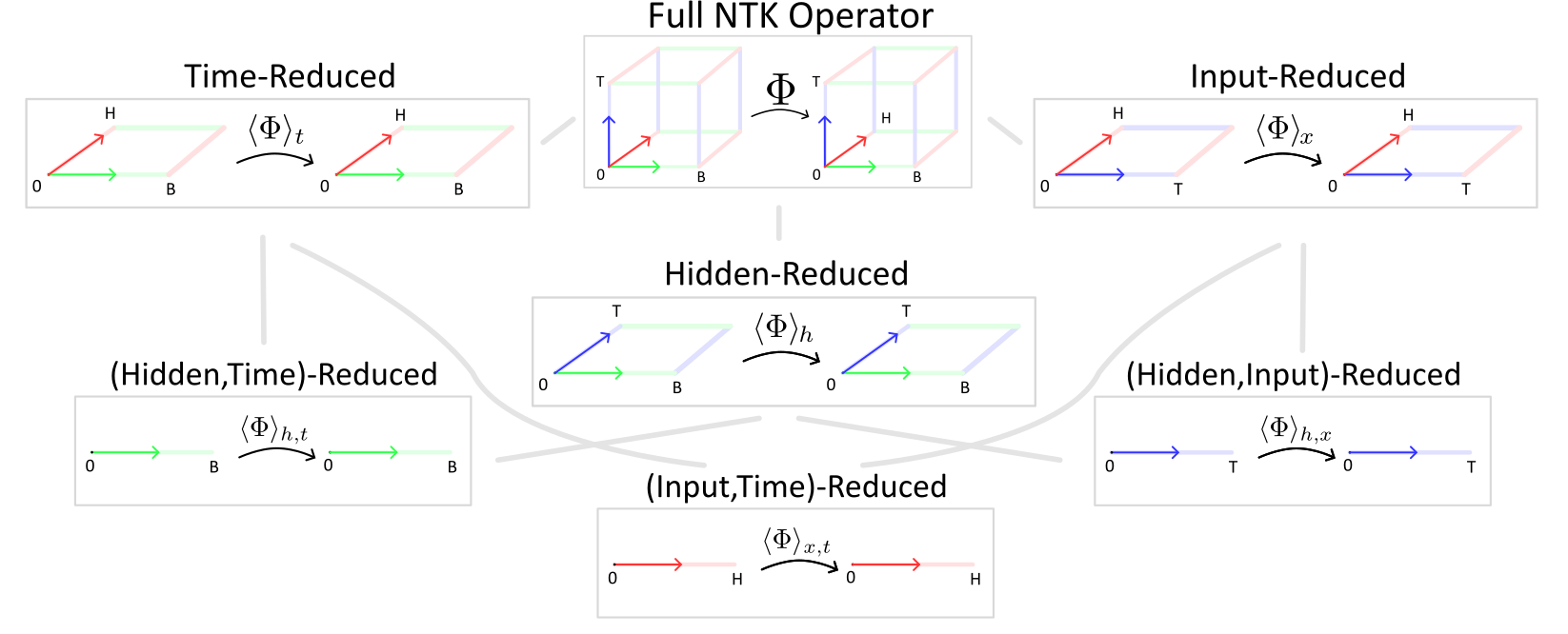
Fig 4 Schematic of heirarchy of views attainable by different reductions of the full hidden-state NTO operator (or related operators).
Reduced Views A simple way to work with this complex operator is to reduce it into simpler "views". The operator itself informs how gradient updates to the hidden state are structured over time, batch inputs and hidden units, which is a ton of information. Sometimes, we would like to know in what subspaces the updates will reside, on average, without consider time or batches. Or, as another example, we want to consider where most of the updates will be concentrated as a signal over time and batches, without thinking about the individual hidden units.
To generate such views, we define a method of reducing the operator over particular axes. Given an axis (time, batches or hidden units), the view of the tensor essentially performs streaming over that axis. For example, let's define the time-averaged NTO \(\langle \Phi \rangle_t\). This is a linear operator now on 2-tensors of shape [B, H]. Specifically, $$\langle \Phi \rangle_t[b, h, b_0, h_0] = \langle \Phi[b, h, t, b_0, h_0, t_0] \rangle_{t, t_0},$$ i.e. we average over the time axes. This operator takes in tensors of shape [B, H], produces a tensor of shape [B, T, H] by making T copies, applies \(\Phi\) to this tensor, then averages the final result over the time axis. In my code, you can find the implementation in op_common.py, called AveragedOperator. Similarly, we can define averaging operations over any of the axes: time, hidden units, or batches, or multiple simultaneously.
Some Example Use Cases
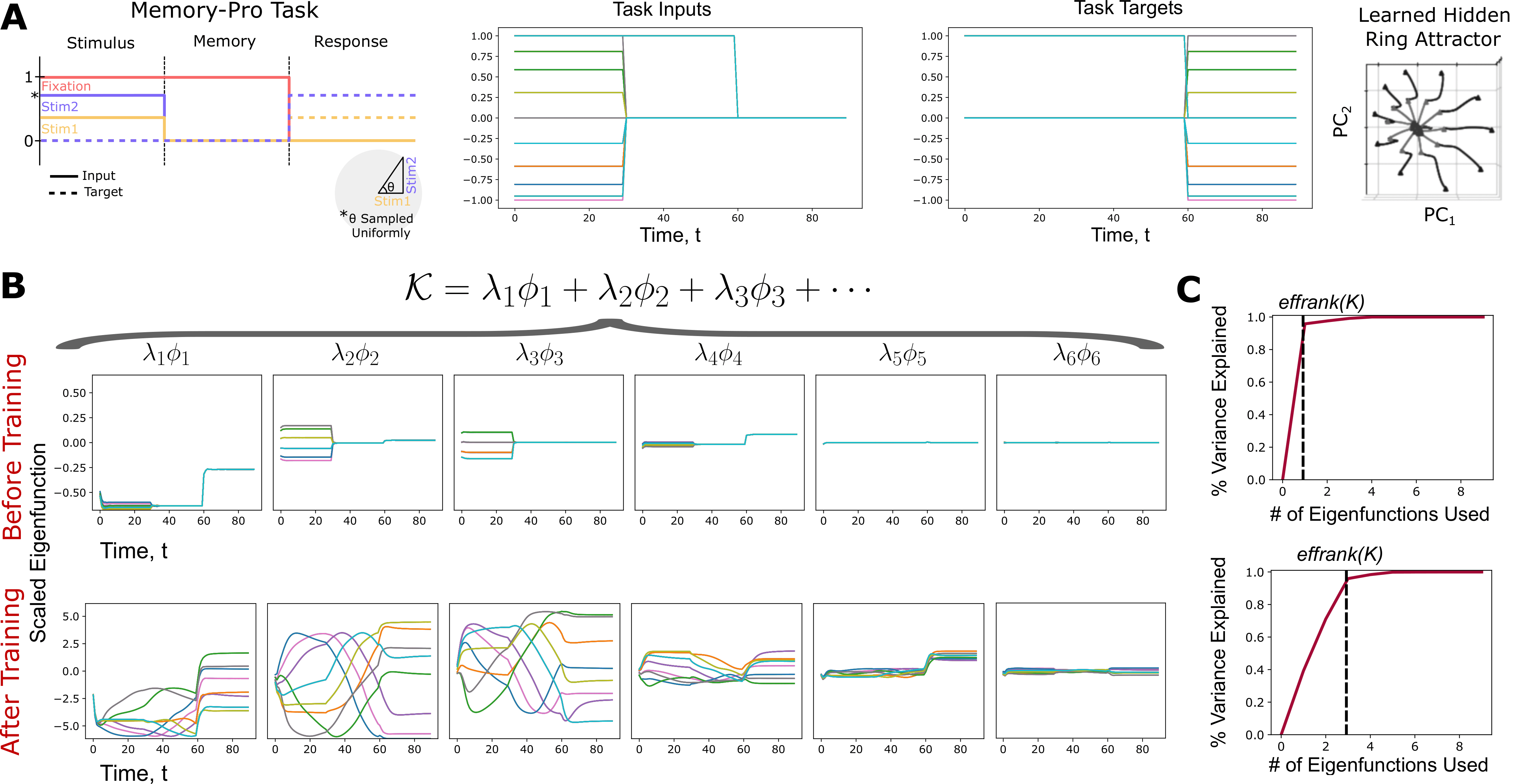
Fig 5 Eigenfunctions and effective rank of the parameter operator \(\langle \mathcal{K} \rangle_{h}\), reduced over the hidden dimension.
As a Matrix Over Hidden Units Using these views, we can measure interpretable properties of the NTO and gradient flow. For example, suppose want to quantify where the gradient updates will be concentrated in the hidden space, irregardless of time or batch trials. Then, we can measure the averaged operator \(\langle \Phi \rangle_{x,t}\), which is now an H by H matrix. We can then measure the singular vectors \(\{v_i\}_{i=1...n}\) of this matrix, and its singular values \(\{\sigma_i\}_{i=1...n}\). The principle vector \(v_1\) explains exactly which types of hidden space inputs will maximally stimulate the operator \(\Phi\), on average over input batches and times. Note that two trials with different inputs, \(x_1, x_2\) to the hidden state, may produce trajectories in completely disparate regions of the hidden space. However, by design, both of these directions will factor in distinctly to the averaged SVD (see my paper Appendix for more explanation of this). If we want to see where gradient updates will be correlated, we can use the left singular vectors, \(\{u_i\}_{i=1...n}\): the first vector \(u_1\) explains where \(\Phi\)'s updates will be contentrated if we given it tons of random input signals, i.e. where GD is likely to concentrate. Finally, the effective rank of the operator \(\langle \Phi \rangle_{x,t}\) explains how hidden space GD updates are constrained: if it is low, it means the operator will be constrained to producing updates in a small, low-dimensional hidden subspace.
Eigenfunction Signals Averaging Hidden Space As another example, we can consider the operator \(\langle \Phi \rangle_{h}\), averaged over spatial hidden units. If we take the SVD of this operator, we get input-dependent eigenfunctions \(\{\phi_{b,t}\}_{b=1...B,t=1...T}\). Each eigenfunction explains which points in time are most crucial to stimulating \(\Phi\), for each individual one of the batch trials. On trial 1, it might say that a particular time window of the task is very crucial, i.e. most of the learning will be concentrated there, while on trial 2, with a different batch input for the model, there could be a completely distinct time window. Consequently, these eigenfunction signals explain the temporal structure imposed by the task on learning, accross each input-driven trial of the model inference. Since the operator is averaged over hidden units, we don't take into account which hidden unit to stimulate, instead we care about which times or indendent input trials are most relevant to the GD update.
Below is a figure more clearly explained in my paper, illustrating the eigenfunctions of the operator \(\langle \mathcal{K} \rangle_{h}\), averaged over hidden units, as in the previous paragraph. A full description of \(\mathcal{K}\) itself is detailed below. The color of each individual trajectory indicate distinct batches. Note that each eigenfunction is a tensor of shape [B, T], as above, informing, on each batch trial, which times are most significant for stimulating the operator. For task setup and more comprehensive details, see the paper itself.
The Full Operator SVD
Simular to the previous use case, we can take the SVD of the full operator, \(\Phi\), without averaging any axes. Then, the eigenfunctions and singular values you get inform how to stimulate \(\Phi\) individually at a very granular level: at each timestep of forward evaluation of the model, hidden unit, and on each distinct input-driven trial.
Decomposing the NTO into \(\mathcal{P}\) and \(\mathcal{K}\)
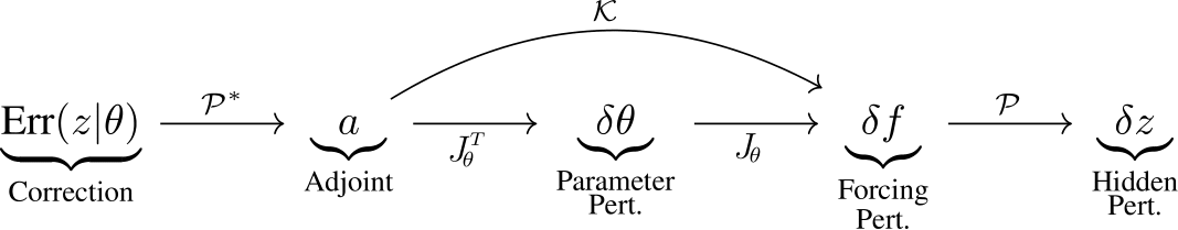
Fig 6 Schematic of the K-P flow decomposition of the full NTO associated with a recurrent dynamical system, as detailed in this blog post.
To summarize the work so far, I have (1) defined the NTO, (2) expained why for recurrent dynamical models it is a linear operator on 3-tensors and (3) discussed how to work with such a weird object. In this section, I will introduce the KP-flow decomposition in my main paper, breaking the recurrent NTO for these general models into a product: $$\Phi = \mathcal{P} \mathcal{K} \mathcal{P}^*$$ where \(\mathcal{P, K}\) are linear operators themselves, which I'll now define, and \(\mathcal{P}^*\) denotes the Hermitian adjoint of the operator \(\mathcal{P}\) (typically just the transpose of the discretized matrix).
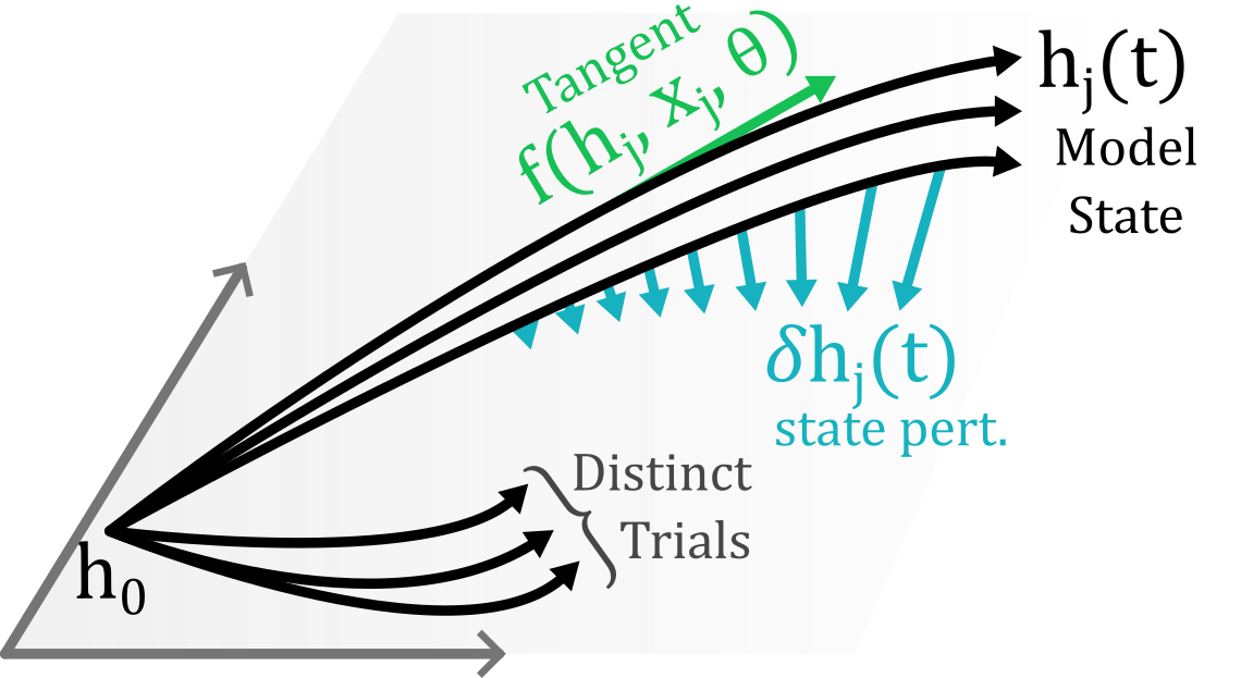
Fig 7 Hidden state trajectories conditioned on the task inputs \(x_j\). The model dynamics \(f\) specify the tangential velocity of each trajectory. Perturbing \(h\) is given as a sequence of perturbations: first the parameters, \(\delta \theta\), then the tangents, \(\delta f\) and finally the state, \(\delta h\).
Consider the model state on task input \(x_j\), which is given by simulating the model from time \(0\) to any \(t\), $$h_j(t) = \int_0^t f(h_j(t_0), x_j(t_0), \theta) \text{d} t_0.$$ Then, there is a chain of perturbations leading to the change \(h_j(t)\) to the hidden state on trial \(j\) at time \(t\). Firstly, there is a perturbation, \(\delta \theta\), to the parameters according to the GD step. Next, this gives rise to a perturbation, \(\delta f\), to the tangential dynamics at every time and trial. When there is a discrete number of timesteps T, H hidden units and B task inputs, \(\delta f\) is a tensor of shape [B, T, H]. Finally, these local changes \(\delta f\) are integrated over time to give rise to the true hidden state change.
In total, there are two constraints on learning:
-
(1) Filtering through parameters meaning that dynamical changes can only be attained by perturbing \(\theta\). Internally, there is a mean yielding this perturbation, which can lead to misdirection or zeroing of gradient signals. For example, if we have a dynamical system with a single parameter, the desired dynamical changes may be very complex, but clearly perturbing a single parameter will not be able to express a very wide range of such perturbations.
-
(2) Local changes emerges from the temporal dependence between the hidden state \(h_j(t)\) and all prior hidden states, \(h_j(s)\). Perturbations \(\delta h_j\) manifest specifically by first perturbing the tangents, \(\delta f\), then accumulating these.
The two constraints described correspond perfectly to the operators \(\mathcal{K}\) and \(\mathcal{P}\). In particular, \(\mathcal{K}\) filters dynamical perturbations through parameters of the model, constraining the range of such perturbations. Furthermore, \(\mathcal{P}\) integrates tangential changes, \(\delta f\), accumulating them into \(\delta h\). Both are linear operators we formally define below. The action of each operator is illustrated in Fig 7 above.
Formal Operator Definitions
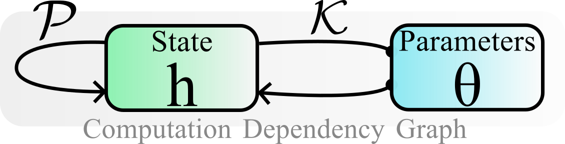
Fig 8 Schematic of computation graph, establishing dependencies in the model. \(\mathcal{K}\) reflects the dependencies emerging from parameters: how do state perturbations filter through parameters, while \(\mathcal{P}\) reflects internal state dependencies.
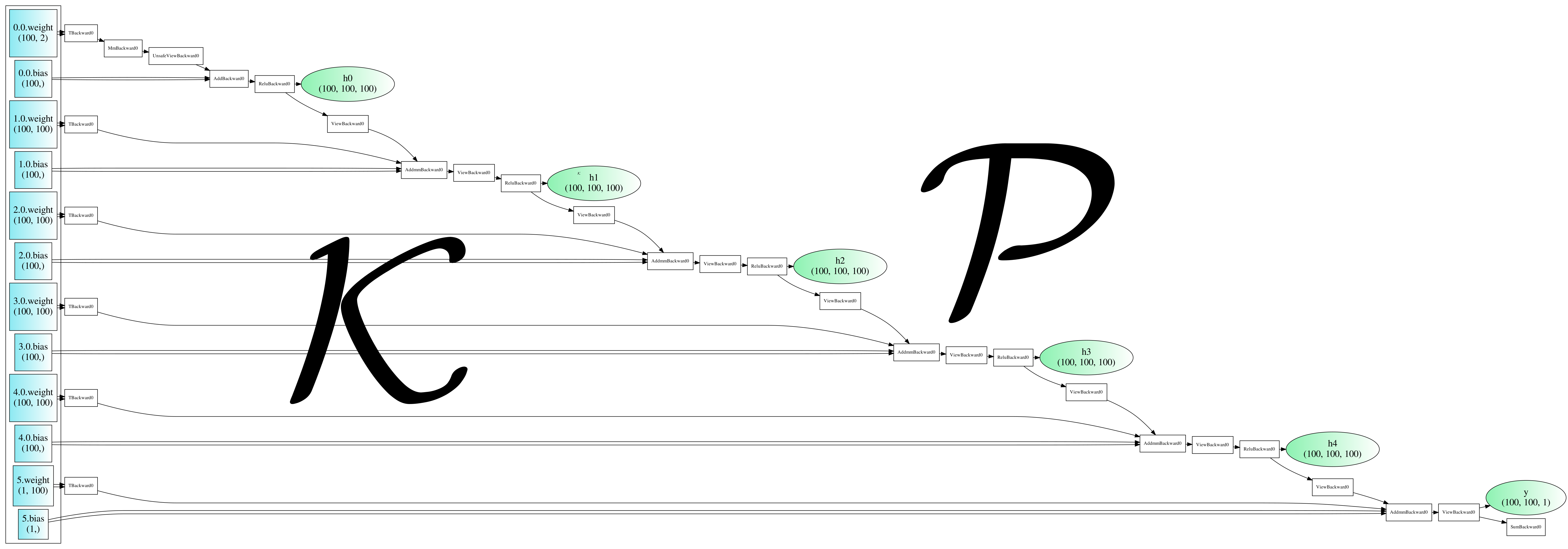
Fig 9 An example computation graph for a discrete MLP neural network with 5 layers of the same size, mirroring Fig 8. The code I used to make such graphs is available with pip! See here or in terminal run "pip install agviz"
Parameter Operator Firstly, let's define the \(\mathcal{K}\) operator, which constrains proposed tangential dynamical updates by filtering these through the model parameters. In particular, \(\mathcal{K}\) is the neural tangent operator for the model velocity, instead of the hidden state itself: $$\mathcal{K} = \frac{d f}{d \theta} \cdot \frac{d f}{d \theta}^T.$$ To simplify notation, we write \(\mathcal{J}_\theta\) for the full tensor. In particular, in the discrete case, assuming the hidden state is a tensor of shape [B, T, H] and \(\theta\) is a vector of length M, \(\mathcal{J}_\theta\) is a [B, T, H, M] with entries $$\mathcal{J}_\theta[b, t, h, m] = \frac{\partial f[b,t,h]}{\partial \theta[m]}.$$ Then, \(\mathcal{K}\) is a discrete matrix with entries: $$\mathcal{K}: \mathbb{R}^{B\times T \times H} \rightarrow \mathbb{R}^{B \times T \times H}$$ $$\mathcal{K}[b, t, h, b_0, t_0, h_0] = \sum_{m=1}^M \mathcal{J}_\theta[b, t, h, m] \mathcal{J}_\theta[b_0, t_0, h_0, m]$$ This is very similar to \(\Phi\), the only difference is that we take the NTO for the model velocity, \(f\), not the overall integrated state, \(h\).
Linear Propagator Next, we define \(\mathcal{P}\), which effectively integrates the results from \(\mathcal{K}\). In particular, given \(\delta f\) perturbing the model tangential velocity, \(\mathcal{P}\) accumulates these, yielding perturbations \(\delta h\) to the hidden state, $$\mathcal{P} : \delta f \mapsto \delta h.$$ First, we define the state-transition matrix \(\Phi_j(t, t_0)\) for the trajectory \(h_j\) on input trial \(j\). Mathematically, it is the Green's function of the model. This measures how small changes, \(\delta h_j(t_0)\), to the hidden state at time \(t_0\) propagate linearly forwards through time to affect the state \(\delta h_j(t)\) at a time \(t\). Specifically, \(\Phi_j(t, t_0)\) is the H by H Jacobian matrix $$\Phi_j(t, t_0) = \frac{d h_j(t)}{d h_j(t_0)}$$ As an aside, the Lyapunov spectra of the model are actually derived from \(\Phi\): if we compute the singular values \(\sigma_i\) of \(\Phi_j(t, 0)\) and let \(\lambda_i = \log(\sigma_i) / t\), then the long-term Lyapunov exponents--describing the long term dynamics of the model on trial \(j\) change if we perturb the initial conditions--are the limit \(\lim_{t \rightarrow \infty} \lambda_i\).
Contrasting this, \(\mathcal{P}\) measures how perturbations propagate at all times and task inputs. Explictly, again in the discrete case where \(h\) is a tensor of shape [B,T,H], \(\mathcal{P}\) has entries $$\mathcal{P}[b, t, :, b_0, t_0, :] = \delta_{b, b_0} \sum_{s = t_0}^t \Phi_b(t, s) \in \mathbb{R}^{H \times H}$$ Note the \(\delta_{b, b_0}\) means that \(\mathcal{P}\) is block-wise diagonal over the batch dimension: perturbations to the hidden state conditioned on two distinct task inputs do not affect one another.
A General Language: Variants of GD in Tensor-Operator Form
Breaking down \(\Phi\) in this form begins to break it into simpler pieces that isolate particular parts of the Backpropagation-Through-Time process. Programmatically speaking, \(\mathcal{P}\) describes the computational graph connections between states, while \(\mathcal{K}\) describes the graph connections from parameters to state.
On one hand, \(\mathcal{K}\) isolates the role dynamical parameters play. For example, if we freeze certain weights during a GD step, the only part of the BPTT pipeline that changes is \(\mathcal{K}\). Furthermore, it can have a simple form for complex models. In my main paper, I found that networks of Hodgkin-Huxley neurons have identical \(\mathcal{K}\) operator structure with a simple vanilla RNN.
On the other hand, \(\mathcal{P}\) isolates the temporal dependencies in the model. If the states did not have temporal dependency, \(\mathcal{P}\) would simply be the identity. Furthermore, complex discrete architectures (e.g. a transformer or network of complex, distinct units) might have very odd dependencies between the internal state. In each case, \(\mathcal{P}\) may manifest in different forms that can be isolated mathematically and in code.
Variants We can describe alternative and similar learning rules using the developed framework. Furthermore, since the operators are implemented in our code, the operators (e.g. their alignment, SVD, rank, etc.) can be compared directly, explictly seeing how different variations of backpropgation align!
-
1. Typical BPTT As above, we have $$\Phi_{bptt} = \mathcal{P K P^*} = \mathcal{P} \mathcal{J}_\theta \otimes_\theta \mathcal{J}_\theta^* \mathcal{P^*},$$ where \(\otimes_\theta\) means "contract parameter dimension."
-
2. Truncated BPTT In the truncated learning rule, the recurrent dependencies between states are not reflected during backpropagation. In particular, the mapping from the error signal to proposed corrections prior to filtering into parameters is simply the identity. Thus, the NTO in this case is $$\Phi_{trunc} := \mathcal{P K}$$ without the operator \(\mathcal{P}^*\) which integrates how the error propagates recurrently due to internal model temporal dependencies.
-
3. Feed-Back Alignment In feedback alignment, the mapping from adjoints, \(a := \mathcal{P^*}(\text{Err})\), to parameter changes, \(\delta \theta\), is replaced by a random matrix \(B_{fba} \in \mathbb{R}^{M \times H}\), assuming M parameters. In particular, the new learning rule is reflected by $$\Phi_{fba} = \mathcal{P J}_\theta (B_{fba} \otimes \text{Id}_{B \times T}) \mathcal{P^*},$$ where the \(\otimes \, \text{Id}\) reflects the fact that \(B_{fba}\) is identical for all batches and times: it is just an M by H matrix mapping hidden states to parameters.
-
4. Functional GD We saw above that there are two constraints on traditional BPTT: (1) local changes and (2) parameter filtering. But we could imagine removing (2), simply kicking each hidden state tangential term in the negative adjoint direction, $$\delta f = -a = -\nabla_h L$$ Unforunately, this is not very useful: it will optimize each individual hidden state trajectory, but it doesn't provide a way of generalizing these changes to the full model. This rule doesn't explain how to generalize the updated trajectories to unseen task inputs. However, we can still define the operator defined by this rule: $$\Phi_{traj} = \mathcal{P P}^*$$
-
5. Gauss-Newton Gauss-Newton is an approach that attempts to implement the functional GD rule above as best as possible, avoiding misdirection due to the operator \(\mathcal{K}\). Recall the pseudo-inverse of a matrix \(A\) is \(A^+ := (A^T A)^{-1} A^T,\) inverting the part that is non-singular. In traditional GD, when you backpropgate you use \(J_\theta^T\). In Gauss-Newton, we instead use \(J_\theta^+\), including the inverse term. In total, this results in $$\Phi_{gn} = \mathcal{P J_\theta (J_\theta^* J_\theta)^{-1} J_\theta^* P^*}$$ We can see the essential idea is to best implement the functional GD by eliminating constrain (2) as much as possible, although typically \(J_\theta\) is singular (there are way more parameters than states), so this isn't perfectly possible.
-
6. Hessian-Adapted Learning Rules As an alternative to forming the pseudo-inverse in Gauss-Newton, we can assume it has some simple form. This is the idea behind methods like k-fac and shampoo. One approach is modelling the Hessian map as a componentwise product in rules like AdaGrad. Updates have the form $$\delta \theta = - v \odot \nabla_\theta L$$ where \(v\) is a vector in the parameter space approximating some second-order Hessian information. Then, the operator is $$\Phi_{adagrad} = \mathcal{P J}_\theta \odot_\theta v \odot_\theta \mathcal{J P}^*$$ Note these learning rules usually take massive steps and rely on stochasticity. We are explictly assuming a gradient flow form, which breaks down when there big GD steps, so that's a limitation. Furthermore, my approach doesn't explictly account for stochasticity in the task inputs, which wouldn't be super hard to add.
As we see in the above, once the tensor-based operators are defined (which is a pain), we can use them to define a language of learning rules. Importantly, for particular models, there are explictly provable properties of the individual operators, as we will see below. Furthermore, we can use the implemented package to implement and efficiently inspect the spectral properties of each operator, isolating how it affects learning or aligns with operators for other learning rules.
Below is an example code snippet from my package, computing eigenfunctions of some operators. Note that you don't need to know all the details above and they're simple to work with!
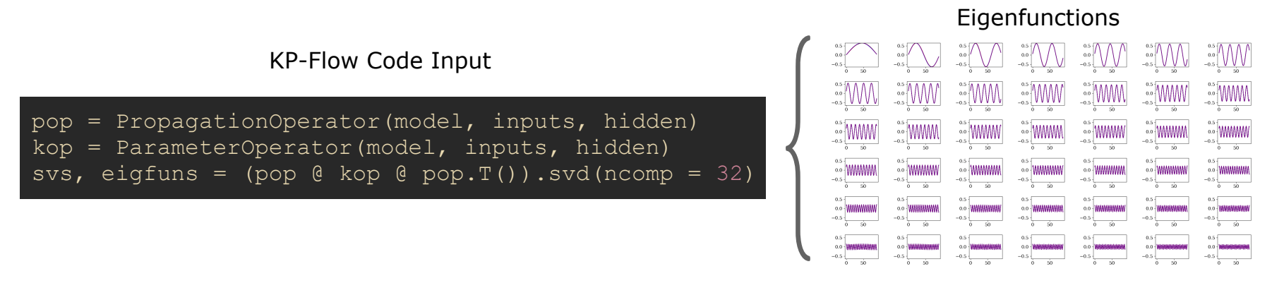
Fig 10 Example code snippet from my kpflow package and plotted (reduced) eigenfunctions.
Finally an Example: Vanilla RNN and Hodgkin Huxley
Application: Simplicity Bias

Fig 11 Simplified version of Fig 6 for reference.
Let's now dig into the innner workings of the operators, their overlap, dominant modes, and the effective rank of their outputs on a particular task. For review, let's define what each quantity means:
-
\(\text{Err}\): The one-step error signal. In the case of MSE loss, \(\text{Err}_j(t) = W_{out}^T (W_{out} h_j(t) + b_{out} - y^*_j(t))\).
-
\(a\): The adjoint signal, \(a_j(t) = \nabla_{h_j(t)} L\). This defines the steepest descent direction at the exact point \(h_j(t)\) in trajectory space. In other words, the exact corrections "functional GD" would produce, if we didn't filter through weights and biases.
-
\(\delta \theta\): The perturbations (e.g., to weights and biases) that GD produces.
-
\(\delta f\): The true perturbations to the one-step dynamics that GD produces due to filtering through parameters.
-
\(\delta h\): The perturbations to the hidden state that GD produces, attained by integrating the one-step changes.
Let's try to characterize these quantities.
Preliminary: Definining Operator Averaged Effective Dimension
Firstly, we need to build a tool for understanding simplicity bias: averaged effective dimension. To understand this, suppose we give an operator \(\Phi\) many random inputs and want to measure the effective dimension of the output \(\Phi q\) in hidden space (averaged over time and batches). To do this We can define the \(H\) average participation ratio dimension as $$PR_H(x) = \frac{x \otimes_{T, B} x^*}{ This motivates a definition $$\text{effdim}_H(\Phi) = \mathbb{E}_x [(\Phi x )
In Progress: Suppose we let \(y = K v\) where \(v \in \mathbb{R}^{B \times T \times H\), \(K\) is an operator on this space. What do we need to do to determine how \(K\) constraints the effective dimension of \(y\), capturing variance over B and T space? To do this, we first form the Grammian $$G_{avg} = y \otimes_{B, T} y^*,$$ where \(y^*\) is a assumed to be the reversed tensor of shape \(H \times T \times B\). Expanding, $$y \otimes_{B, T} y^* = (K v) \otimes_{B, T} (v^* K^*)$$